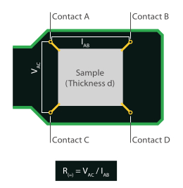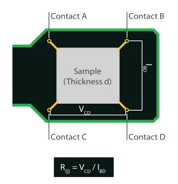
Zur Bestimmung des spezifischen elektrischen Widerstands (oder der elektrischen Leitfähigkeit) der Probe wird die Van-der-Pauw-Messtechnik verwendet. Dadurch können beliebig geformte Proben analysiert werden, störende Einflüsse wie Kontakt- oder Drahtwiderstände werden unterdrückt und die Messgenauigkeit kann deutlich erhöht werden.
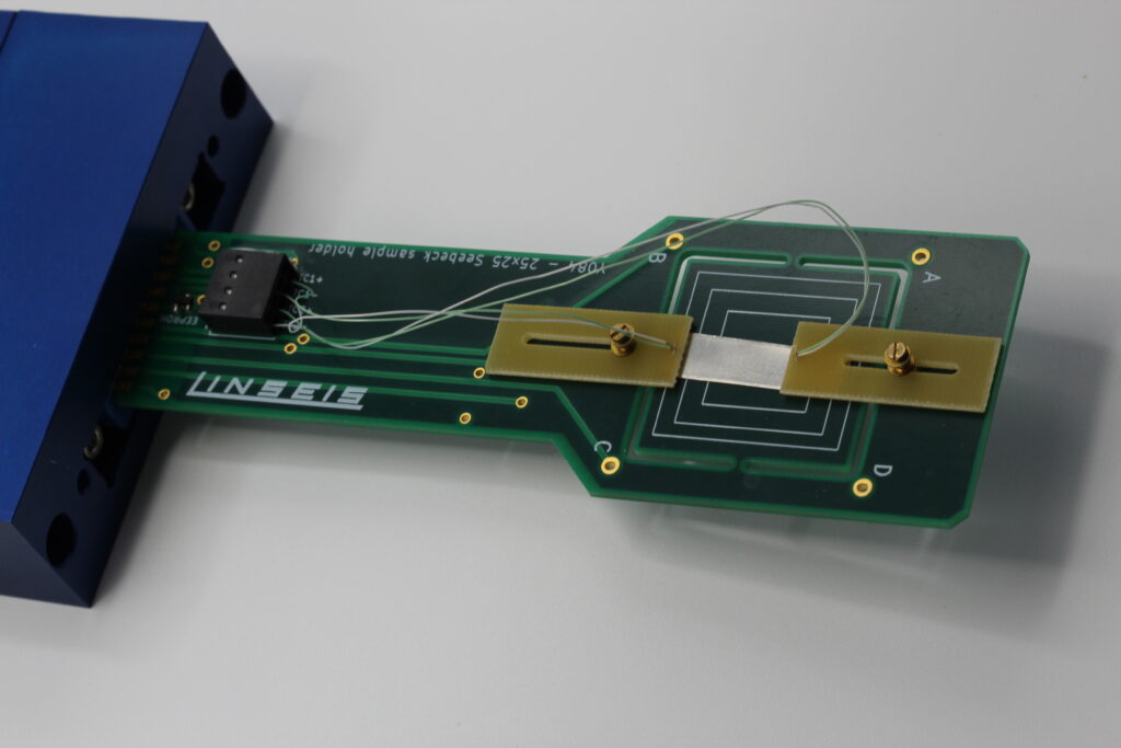
Für die Van-der-Pauw-Messung muss die Probe mit vier Elektroden direkt an der Kante verbunden werden. Im ersten Schritt des Routings wird an zwei Kontakten an einer Kante der Probe ein Strom zum Fließen gebracht und die Spannung an den beiden anderen Kontakten an der gegenüberliegenden Kante gemessen. Aus diesen beiden Werten lässt sich mit Hilfe des Ohmschen Gesetzes ein Widerstand ermitteln. Im zweiten Schritt werden die Kontakte zyklisch geschaltet, und die Messung wird wiederholt. Der Schichtwiderstand der Probe kann dann leicht berechnet werden, indem die beiden gemessenen Widerstände (horizontal und vertikal) in die Van-der-Pauw-Formel eingesetzt und gelöst werden.
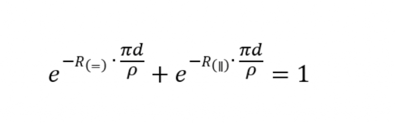
Ausgehend von den gemessenen Daten und dem Thermoelementabstand “t” können der spezifische Widerstand und die elektrische Leitfähigkeit nach folgenden Formeln berechnet werden: